Selecting Areas Using the Query Table

Selecting Areas Using the Query Table
1. Open ArcView GIS 3.3
2. Open Project which we created earlier
3. Click the Theme then select Table ...

4. The image will appear like the one below, which contains vast area and is concerned with the data on the map

5. Click the QUERY BUILDER as shown below

6. Query window will appear which can be applied to select the data in the table map
7. For use here as a connector AND a second prerequisite conditions must be met. For example, type the command "(([Area] <= 500 000) and ([Perimeter]> 4000) then press New set

8. Images on the map will be selected by the condition of the area must be less than or equal to 500 000 and must have a perimeter greater than 4000

9. To use OR here as a condition where one of the conditions to be met. For example, type "(([Area]> 20000) or ([Perimeter] <5000))"

10. In the map will be selected all because of one or all of the conditions are met

11. NOT for use as a condition rather than in specific terms. Type "not ([Area] <400 000)"

12. The result is only one who is not selected because the area has an area of less than 400 000

Read More

Convert Line to Polygon using MNDNR and Edittool (ET)

Convert Line to Polygon using MNDNR and Edittool (ET)

line-to-polygon

For digitizing a map we need accuracy and precision in making the boundary line. However, the weakness of the line or polygon is very difficult to make a line corresponding to the lines on the original map. On this occasion I will show you how to makes a polygon using a line that was converted into a polygon polyline later. First and foremost we have to add the extension (ext) in the form MNDNR Stream Digitizing form and Edit Tool (3.1) or can be downloaded here.
1. Open the map and turn on the necessary extensions like MNDNR, Edit tool, and JPEG
2. Create a new theme by clicking view&gt; New Theme then the type was replaced by Line
3. Click the Open Stream Digitize Form Strean then click Digitize line as shown below

line-to-polygon 3

4. Create a line as it is on the map. To get started click on the map and then drag the mouse. To complete the double click.
5. Set the scale used map view by clicking&gt; Properties ...
6. Set the map units to decimal degrees and distance units to kilometers according to the picture below

line-to-polygon 6

7. Click the ET icon on the toolbar, click edit theme, and select a theme that we have made before, or can be seen as below

line-to-polygon 7

8. To check whether the line we are well ordered by clicking the edit button clean on the toolbar, and then click the full and click the Intersect. Wait until the process is complete.

line-to-polygon 8

9. To correct and edit the line that we can use the tool by clicking the Edit tool on the toolbar view edit tool first appeared.
10.Setelah everything was in place, use a clean check back if there are any left or not. If not we will proceed to the next process
11.Setelah finished editing click the stop button, then click the Build Polygons beneath it.
12.Tunggu until the process is finished, a quote for temporary storage and click OK. If successful will appear back window to save the polygon that has been so.
13. After finishing the previous lines we make will be colored. to make a difference in the color of each region by double clicking polygon theme. Then change the Legend Type to "Uniquw Value" and Field "ID" then click Apply.

Read More

LayOut

LayOut

LayOut

In a digitized map of the last one we did was print out a map that has been digitized, here are the steps to create a digitized map into a neat layout-layout and can be read by lay people
1. Open the application ILWIS 3.3 Academic
2. Open the tab Clip_Slope_pct raster map
3. It would seem that we have digitized maps previously
4. Back to the main window and then right click Clip_Slope_pct> vectorize> Raster to Polygon ...
5. Give the name of the output with Slope_PCT> Show> OK
6. Replace the yellow color 0-10> 10-20% also replace the color orange> Orange Red 20-40 to> 40-60 a light green >> 60 to Grey> OK
7. 0-10 Area will change to yellow and so on
8. Click Layers> Add graticule ...
9. replace graticule distance to 0 0'45 "and the color becomes DodgerBlue> OK
10. then you will see the lines as coordinates of the map that we will print later
11. add grid is also a way to Layer> Add Grid Lines ... > Provide grid distance: 2000.000> OK
12. uncheck the grid if you want to eliminate the lines of the existing grid
13. Click File> Save View> Enter the name of the Slope> OK
14. Object Collections Click on the toolbar at the top of the Command Line
15. Slope Right Click> Create layout ...
16. Fill Scale 1: 25000> OK
17. Maps that have been digitized image will appear on the paper> Position and resize to fit the paper
18. Click File> Page Setup> change the paper size according to the paper you use to print the map
19. Click Insert> Legend ...
20. Add a check on the Bold and change the font size to 14 for easy reading later> OK
21. Add also the north of the map by clicking Insert> North Arrow
22. Replace radio check with Compass: 8 and Bold> OK
23. Include the scale used by Click Insert> Text Scale> turn bold> OK
24. Enter Scale bar is also in the same way is to click Insert> Scale bar> Fill Unit needs to be included as Indication, Use Km, Bold and the interval to 3> OK
25. Do not forget to enter the border map that maps better and easier to coordinate readings by clicking Insert> Folder Border> change tab to graticule and a check pad graticule Coordinates> switch to full coordninate and color into dodgeblue> Text Offset: 6> OK
26. It will be seen next to the map coordinates
27. Add Text icon by clicking the "Abc" on the toolbar and enter the text according to your project, for example, UTM PRJ Map
28. For our direct print then click File> Print ...
29. But when will we export into the image by clicking File> Export to Bitmap ...
30. Give it a name that suits Slope atupun you want> OK
31. Close the project and save it with the same name
32. The images we have made will be in the directory that we specify


For more details see the following video tutorial
PART 1
PART 2 or can be downloaded here

DOWNLOAD

Read More

Data Control

Data Control

Data Control

1. Open the application ILWIS 3.3 Academic
2. Open Hipsometery on tap Raster map
3. Add layer by clicking the Add Data Layer> select topo> OK
4. a check on the Mask and fill in the * 00.0001> replace radio checks with Single color> select color black> OK
5. It will then appear with a black line topology
6. Back to the main window and then click open Aspect_flat_nine
7. Add the data layer by clicking the Add Data Layer> select River_code> OK
8. Add thickness streams by clicking a "1" on the sub Legend> replace Line Width to 0.8, did on another stream line ("2", "3")
9. Double click on Aspect_flat_nine on the left screen
10. replace radio checks on Grey> OK
11. The color of the topology will turn gray and the lines will appear River


For more details see the following video tutorial

or can be downloaded here

DOWNLOAD

Read More

Extract information for Physiography Report

Extract information for Physiography Report

Extract information for Physiography Report

1. Open the application ILWIS 3.3 Academic
2. Open the tab back_ground raster map
3. Add layer by clicking the add layer data> catchment_boundary> OK> OK
4. Click Edit> Edit Layer> 2 seg catchment_boundary
5. Snap and tunnel tolerance to 0 at File> customize ...
6. Draw a line to the tool insert mode in accordance with the lines on the map
7. When there are warning Splite segme ... then select OK
8. After completion will appear lines are interconnected at the border on the map
9. Click File> Polygonize ... > Insert the name of the output with Sub_base> add domain and enter the name of the Sub_base> OK> OK
10. If there is a warning only segments select YES
11. Bring segment (more details to see video)
12. Dead End To check whether or not there is a way> File> Check SEGMENTS> Dead Ends ... > OK> If a warning has shown no dead ends is not there then we proceed to the next step if there is to be checked again
13. File> polygonize ... > Insert the name of the output with Sub_base> insert domain with sub_base that we created earlier> OK
14. Click the area you will be given the name of the> class name> New> insert name and color with a red> OK
15. Fill up all over the place colored
16. Do not forget to always keep the project
17. Right click on the tab Sub_base polygon map> select Polygon to Raster ...
18. Fill GeoReference with Best_GeoRef that we created earlier> Show> OK
19. Right-click the tab Sub_base existing raster map> select Raster Operations> Cross ...
20. 2nd Map: Aspect_Flat_nine> Output table: aspect_Sub_base> Check the list on the Output folder> Output folder: aspect_Sub_base> OK> table will appear on the data aspects of the sub base that we created
21. Perform the operation again cross between sub_base with clip_slope_pct, right click Sub_base> Raster Operations> Cross ...
22. 2nd Map: clip_slope_pct> Output table: Slope_Subbase> Check the list on the Output folder> Output folder: Slope_Subbase> OK> will appear on the data table slope on the sub base that we created


For more details see the following video tutorial

or can be downloaded here

DOWNLOAD

Read More

Gravity Center

Gravity Center

Gravity Center 

1. Open the application ILWIS 3.3 Academic
2. Open catchment in raster map
3. Right click on the catchment> vectorize> Raster-to-point ...
4. Fill output catchment_point> show> OK
5. Constituent picture will emerge with the points very much
6. Open the tab catchment_point point folder> right click and select Open as table
7. Click View> command line, to bring up the command line
8. Type X = CRDX (Coordinate)> OK
9. Will munucul new column that contains X
10. Type Y = CRDy (Coordinate)> OK
11. Click on view> statistics Pane
12. Back to the main window and then click File> create> Table
13. fill in the name of the table with G_Center> Record: 1> OK
14. add columns by clicking Columns> add column
15. Fill in the name of the column with X> OK
16. Add a column and named Y
17. Back to the table and then copy cathment_point Average X by right click> copy or CTRL C
18. And paste it into the table G_Center in column X
19. Do it again on the Y, Y Average copy and paste the table into catchment_point Y column in the table G_Center
20. Go to the main window and then click the folder table located above the command line and right click on G_Center> Table Operations> table to PointMap ...
21. Select the Coordinate System UTM_WGS1984
22. Enter the G_Center Output> Show> OK
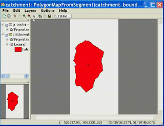
23. Open the file Catchment Polygon map> add layer by clicking the Add layer and add G_Center
24. The result will be the mid-point of the polygon catchment is on the screen


For more details see the following video tutorial

or can be downloaded here

DOWNLOAD

Read More

Profile (River Profile)

Profile (River Profile) 

Profile (River Profile) 

1. Open the application ILWIS 3.3 Academic
2. Click the Segment folders on the toolbar above comment Line
3. It would appear that type of file segments only
4. Right click on the River> vectorize> Segment to Point ...
5. Click the radio and moved to distance> 5.00 and fill fill point with River_point Output> Show> OK
6. On the screen will appear showing the circles of the river segment
7. Add layer by clicking the add layer> then enter the river> OK> OK
8. Then return to the main window> Click on Point folder> Right Click River_point> Open as Table
9. It would appear all the data on the coordinates in the stream segmentation
10. Type the command into the command line Distance = (% e-1) * 5> press Enter> OK
11. It would appear that our new column named distance was
12. Type the command into the command line ALTITUDE = MapValue (DEM_av.mpr, coordinate)> OK
13. Emerging new table will appear on Altitude
14. To display the statistics click View> Statistics Pane
15. Will appear min, max, average, standard deviation, and sum
16. create graphs by clicking on the Graph toolbar menu located on the command line
17. Fill in the X-Axis and Y-Axis Distance with Altitude> OK
18. Graph will appear
19. Back to the table and then type in the command line with Area = altitude * 5> press Enter> OK

For more details see the following video tutorial



or can be downloaded here

DOWNLOAD

Read More